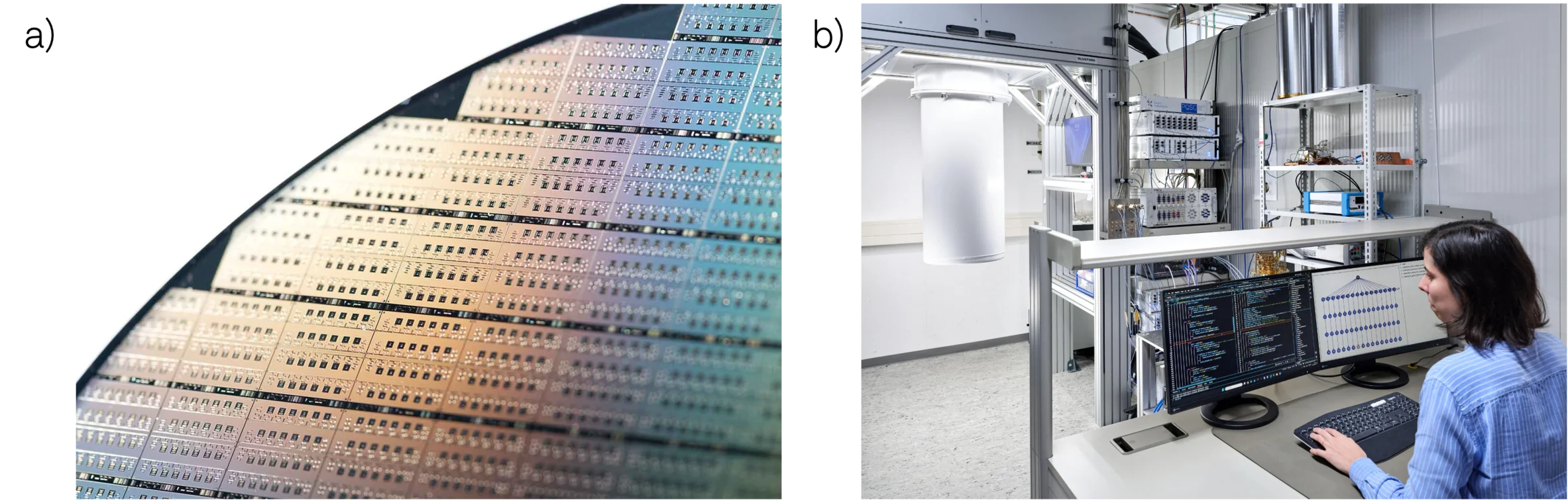
Automated Qubit Bring-up with LabOne Q: From Design Parameters to Identified Qubits
Getting superconducting qubits from fabrication to first useful data is time-consuming. Days of cooldown are followed by hours of careful spectroscopy, manual power sweeps, and resonance hunting - repeated for every new chip. As the quantum computing industry matures and fabrication throughput increases, this manual characterization process - also called bring-up - becomes an increasingly significant bottleneck.
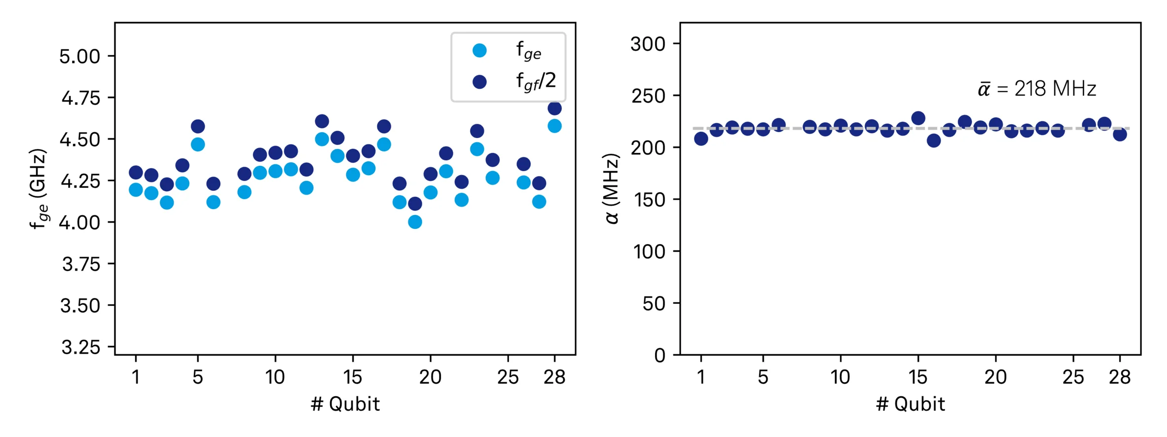
Our automation framework based on LabOne Q addresses this challenge directly, taking newly fabricated qubits from design parameters to fully characterized devices with minimal human intervention. In our collaboration with Fraunhofer EMFT, we put this workflow to the test on seven 4-qubit chips. The system successfully characterized all 28 qubits in approximately 3 hours of total runtime - a dramatic reduction compared to manual approaches that would typically require days of operator time for the same set of devices. Two qubits exhibited very weak coupling and were flagged correctly by the framework, all remaining 26 qubit were identified and characterized.
The Case for Automation
Automation dramatically reduces the time from cooldown to first data by eliminating repetitive discovery routines. Furthermore it encodes best practices and decision logic into the workflow itself, making the system robust against device variability without requiring constant expert oversight. Third, it enables parallel execution across qubits and chips where crosstalk permits, providing a path to scale as device complexity grows.
The question isn't whether to automate, but how to do it in a way that handles real-world device variability while remaining flexible enough to adapt to different chip architectures and user requirements.
Workflow Architecture: The DAG Approach
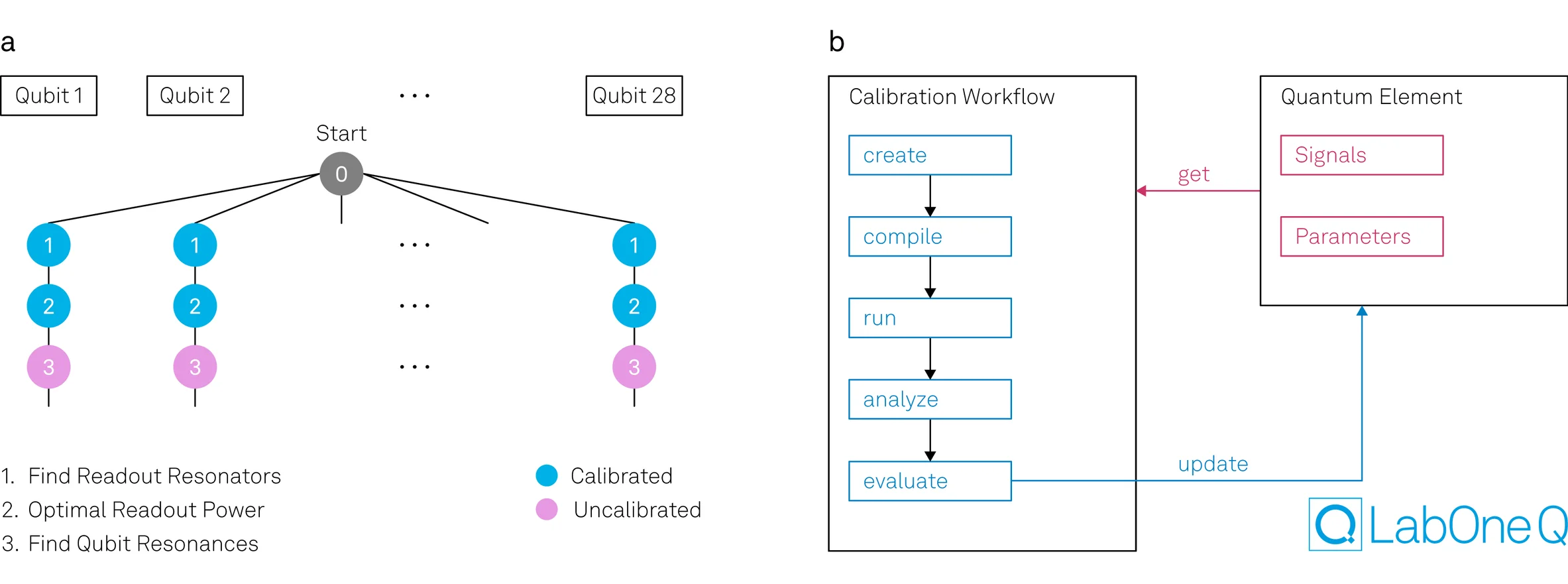
We organize the bring-up process as a directed acyclic graph (DAG), which provides natural orchestration for complex measurement sequences. Each node in the graph represents a complete calibration workflow that follows a consistent pattern: initially, the system creates, compiles, and executes an experiment using the best available parameters at that moment. These parameters might be previously measured values - such as a readout resonator frequency identified in an earlier step or design parameters drawn from the device design when no measurement data exists yet.
Once the experiment runs, the workflow analyzes the acquired data and evaluates whether the calibration succeeded according to predefined criteria. Success might mean detecting a resonance above a certain signal-to-noise threshold, or identifying a spectroscopic feature with sufficient confidence. When a calibration succeeds, the workflow updates the known parameter set with the newly measured value. If a calibration fails, the system can flag the issue, attempt recovery strategies, or stop and mark that particular qubit or coupling element for manual follow-up. This cycle - measure using current knowledge, analyze, validate, and update - repeats at each node, with the parameter set becoming progressively richer as the workflow advances through the graph. Our architecture cleanly separates data acquisition, analysis, and decision making while it maintains while maintaining flexibility to add, remove, or modify steps without restructuring the entire workflow.
The DAG framework lets you optimize execution strategies even further. Results from each node are cached, allowing rapid re-runs when only a subset of parameters change. Dependencies are tracked automatically, so the system knows which downstream steps need to be re-executed and which can use cached results. This becomes particularly valuable during development and debugging, where you might just iterate on a single step.
Exerimental Validation: From Design Parameters to Identified Qubits
We validated this workflow on seven chips from Fraunhofer EMFT, each containing four qubits in a single-feedline architecture where drive and readout signals share the same transmission line. The measurement setup comprised an SHFSG8 Signal Generator for drive and an SHFQA4 Quantum Analyzer for readout. With the SHFQA4's four I/O channels, we could connect up to four chips simultaneously, enabling parallel measurements across up to sixteen qubits at once - a capability that proved crucial for achieving our 3.5-hour total runtime.
The bring-up process progresses through four main stages, each building on the results of the previous steps. We begin with resonator spectroscopy, scanning a frequency tone across the expected readout bands. The analysis pipeline applies a peak finder to identify resonator candidates, using quality factor and signal-to-noise ratio as discriminating metrics. In single-feedline architectures like these, multiple resonators share the same transmission line, making efficient parallel sweeps essential for throughput. Here, our parallel execution capability shines - we performed resonator spectroscopy simultaneously across all four connected chips, characterizing sixteen resonators in a single sweep.
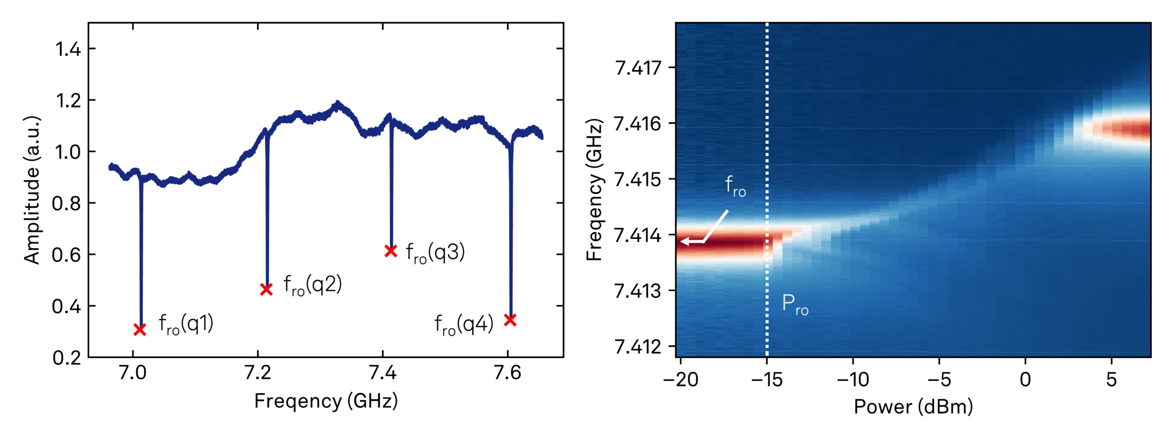
Once we've detected resonator features, the next challenge is attribution - determining which resonator corresponds to which physical qubit. The workflow uses design parameters including nominal ordering, coupling layout, and expected frequency spacings to map each detected resonator to its intended qubit. This automated attribution proved particularly robust in our tests, successfully handling the resonator frequency spreads we observed across chips. The fabrication variability was relatively small in this case, but the attribution algorithm is designed to handle larger permutations when necessary.
With resonators identified and attributed, power-dependent resonator spectroscopy provides our first test of qubit viability. By sweeping readout power and tracking dispersive shifts in the resonator response, the system infers qubit-resonator interaction strength. A functioning qubit will shift its resonator frequency under measurement drive through the dispersive interaction; a non-functional device won't produce this signature. This step delivers a binary classification - alive or not alive - for each qubit, allowing us to focus subsequent efforts on viable devices. Additionally, we extract a first estimate for the optimal readout power Pro for each qubit using a straightforward heuristic: we select the maximum power just before the dispersive shift saturates, balancing signal strength against potential qubit heating or nonlinear effects.
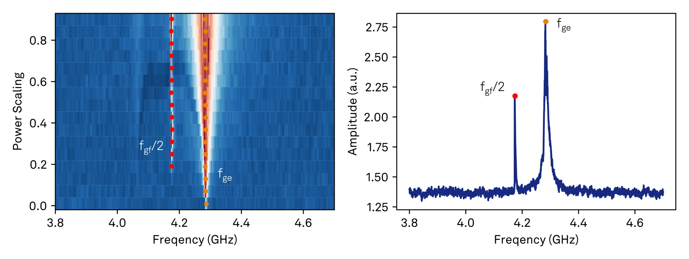
The final stage is qubit spectroscopy itself. We sweep drive frequency and power while monitoring the readout response, then apply peak-cluster analysis across power levels to identify stable resonances. This analysis targets both the fundamental |g⟩→|e⟩ transition and the lower anharmonic transition at (|g⟩→|f⟩)/2. Given that qubit frequencies can exhibit substantial spread relative to design values, this calibration step includes automatic escalation strategies. If the initial scan around the design frequency finds no resonances or only a single peak, the workflow automatically shifts the search window by half its width and repeats the measurement. This process continues in windows progressively further from the design frequency until either both expected resonances are identified or the entire allowed frequency range has been scanned. This adaptive approach can save time while still allowing the system to either locate difficult devices or definitively flag them for manual investigation.
Total runtime was approximately 3.5 hours, with the first four chips taking about 2 hours and the remaining three chips completed in 1.5 hours. This improvement reflected both parameter convergence as the system learned typical device characteristics and increased parallelization efficiency on later runs.
Results and Performance
The automated workflow successfully characterized 26 of the 28 qubits across all seven chips, extracting a complete set of bring-up parameters for each device: readout resonator frequency, optimal readout power, qubit transition frequencies fge and fgf/2, and anharmonicity. The total runtime was approximately 3.5 hours: 2 hours for the first four chips and another 1.5 hours for the remaining three.
The two qubits that the workflow couldn't fully characterize proved instructive rather than problematic. Both exhibited very weak coupling, which we confirmed through follow-up manual measurements. This represented genuine device outliers rather than a failure of the automated workflow. The system performed as designed: it systematically increased drive power through its escalation strategy, reached the limit, correctly flagged low signal quality and marked the device for manual investigation. These edge cases demonstrate the workflow's ability not just to characterize typical devices, but to identify and communicate when a device or experimental condition falls outside expected bounds.
Note: The DAG framework in general enables parallel execution of calibration workflows across qubits and chips, but the single-feedline architecture often requires sequential scheduling to avoid unintended cross-drive and readout collisions. Using independent drive lines, the parallelization constraints relax and throughput can increase substantially. The DAG framework adapts to these different architectures, allowing the same workflow logic to operate efficiently across different device geometries.
Intelligent Automation
What distinguishes this workflow from simple scripting is the intelligence embedded throughout. Each node in the DAG accepts user-configurable settings - e.g. frequency ranges, power ranges, resolution, averaging, and thresholds for evaluation. Default values enable hands-off operation for standard cases, while expert users can override parameters for specific qubits or chips when needed. This per-step, per-qubit parameterization provides the flexibility to handle edge cases without requiring custom code for unusual qubits/chips.
Beyond static configuration, the framework adapts its behavior based on intermediate results through escalation strategies. The qubit spectroscopy step demonstrates this in action: when the initial scan around the design frequency finds no resonances or only a single peak, the workflow automatically shifts the search window by half its width and repeats the measurement. This process continues in windows progressively further from the design frequency until either both expected resonances are identified or the entire allowed frequency range has been exhausted. This adaptive search proved essential for locating qubits with significant frequency deviations from their design values.
The escalation concept extends naturally to other scenarios. When signal-to-noise falls below a threshold, the system can automatically increase averaging. When a spectroscopic feature appears narrower than the initial sweep resolution, it can refine the scan in that region. While we haven't implemented every possible escalation strategy in this demonstration, the framework provides the hooks to add them as needed. These decisions execute automatically, guided by detection confidence metrics and predefined thresholds that can be tuned based on accumulated experience with a given fabrication process.
Over time, the workflow becomes a repository of institutional knowledge - encoding the tricks, heuristics, and recovery strategies that experienced operators develop through repeated interaction with a device family. Rather than requiring each new operator to rediscover these best practices through trial and error, the automation captures and applies them consistently across all measurements.
Extending Toward Complete Tune-Up
This bring-up workflow establishes the foundation for complete device characterization. The modular DAG architecture naturally extends to include Rabi amplitude and DRAG parameter extraction, readout discrimination and threshold calibration, coherence measurements including T₁, T₂, Ramsey, and echo sequences, and flux bias sweeps for sweet-spot detection. Each additional characterization step becomes another node in the graph, consuming calibration parameters from bring-up and emitting refined parameters for gate-level operations.
The workflow thus grows with your needs. Standard characterization nodes can be incorporated from a library, while custom steps can be added for specific device architectures or research questions. As a reference, you can also view our published application note on automated tune-up for Transmon Qubits, which provides another example for building extended workflows using our automation framework.
Acknowledgments
We thank Fraunhofer EMFT for providing the qubit chips and their active collaboration on validation measurements within the MuniQC-SC project. We thank the Walther-Meißner-Institut for providing access to their experimental setups during the development of the automation framework. We gratefully acknowledge the support and funding by the German Federal Ministry of Research, Technology and Space (BMFTR) received for the MuniQC-SC initiative. The funding was instrumental in conducting parts of the work detailed in this blog post. Finally, we want to thank Benedikt Lezius for his tremendous help and contributions to the workflows utilized in this work.
If you're interested in the example DAG implementation, workflow templates, or discussing how to adapt this workflow to your specific setup, please get in touch. We're happy to share implementation details and learn from your characterization challenges.