Measuring the 1st, 2nd and 100th Derivative with Lock-in Amplifiers

Let’s be clear: there is (probably) no physical use case for measuring the 100th derivative – and the signal would be very weak – but mathematically it is possible, hence the title.

Detecting current or voltage while sweeping an experimental parameter is a common technique in many applications, for example for:

• Characterization of materials, solar cells, and low-dimensional devices: urrent is measured as a function of an applied DC voltage.
• Magnetometry using ensembles of Nitrogen-Vacancy centers: Fluorescence intensity is measured via current from a photo detector as a function microwave excitation frequency (optically detected magnetic resonance (ODMR)).

In both examples, the signals are often very small and buried in noise; thus, precise measurements are only possible by modulation of an experimental parameter and demodulation using lock-in detection. The modulation can be applied to different parts of the setup. In the two examples above, it is possible to directly apply a modulation to the sweeping parameter: for measuring current as a function of voltage, a small AC voltage can be added while sweeping the DC voltage, while a frequency-modulated excitation signal can be used for ODMR measurements. Using a lock-in measurement at the modulation frequency ω, one is then measuring relative changes of the measurement parameter, e.g. ΔI instead of the DC current I.

Differential conductance measurements

Let’s look at measurements of current as a function of voltage (so-called IV curves) in more detail and convince ourselves that demodulation of the modulated experiment gives the differential conductance (dI/dV) as a function of voltage. This is not only advantageous in terms of the signal-to-noise ratio of the measurement, but in many experiments, the underlying physics is also easier to observe in the differential conductance; for example, when studying charge states of quantum dots where a new transport channel is resulting in a discrete step in the differential conductance.

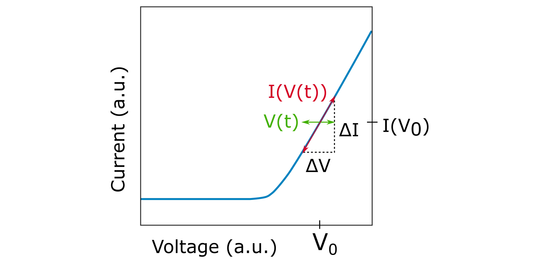
But why does the demodulation give the derivative? Let’s look at the math behind it. Figure 1 shows an IV curve of an LED, which was measured by sweeping the DC voltage and measuring the DC current (this blog post shows how to set up a DC measurement with the MFLI Lock-in Amplifier). Let’s focus on the measurement at V₀. If we modulate the voltage V(t) = V₀ + Asin(ωt), the resulting current I(V(t)) will also be modulated. A lock-in measurement at frequency ω gives the amplitude of the current modulation – and visually it can be understood that this corresponds to the derivative of the current at V₀, that is dI/dV at V=V₀.

Mathematical derivation with the Taylor expansion

For the mathematical explanation, let’s recall the Taylor expansion:

\[ f(x_0+x) = f(x_0) + \frac{f'(x_0)}{1!}x + \frac{f''(x_0)}{2!}x^2 + \cdots \]

Now we can write I(V(t)) as the Taylor expansion:

\[ I(V(t)) = I(V_0 + A\sin(\omega t)) = I(V_0) + \left.\frac{dI}{dV}\right|_{V_0} A\sin(\omega t) + \left.\frac{d^2I}{dV^2}\right|_{V_0} \frac{A^2 \sin^2(\omega t)}{2!} + \cdots \]

Using sin²(x)=(1-cos(2x))/2, it follows

\[ I(V(t)) = I(V_0) + \left.\frac{dI}{dV}\right|_{V_0} A\sin(\omega t) + \left.\frac{d^2I}{dV^2}\right|_{V_0} \frac{A^2}{4} - \left.\frac{d^2I}{dV^2}\right|_{V_0} \frac{A^2}{4}\cos(2\omega t) + \cdots \]

Measuring the 1st derivative

With the lock-in amplifier, we can now filter out certain frequency components. Doing a demodulation at f=ω corresponds to filtering out only the terms containing a sin(ωt) term, and the demodulated result is therefore:

\[
\text{DemodR}_{\omega} = \left.\frac{dI}{dV}\right|_{V_0} A
\quad\Longrightarrow\quad
\left.\frac{dI}{dV}\right|_{V_0} = \frac{\text{DemodR}_{\omega}}{A}
\]
 

Which confirms that the derivative dI/dV can directly be measured by demodulation at the modulation frequency ω.

Measuring higher derivatives

If we do the demodulation at f=2ω, only the terms containing cos(2ωt) remain after the low-pass filter, and therefore:

\[
\text{DemodR}_{2\omega} = -\left.\frac{d^2I}{dV^2}\right|_{V_0} \frac{A^2}{4}
\quad\Longrightarrow\quad
\left.\frac{d^2I}{dV^2}\right|_{V_0} = -\frac{4\,\text{DemodR}_{2\omega}}{A^2}
\]

Note that because it was a cos(2ωt) term, the signal will be in the Y quadrature. 

What does this mean for the 3^rd, 4^th and 100^th derivatives? If we look at the Taylor expansion, we can observe that there will always be a term containing sinⁿ(ωt). This can be expressed as a series of terms, including a term of dⁿI/dVⁿ*sin(nωt) (or dⁿI/dVⁿ cos(nωt)), which means that it is possible to measure dⁿI/dVⁿ by demodulating at the n^th harmonic. However, the n^th term scales with n!, meaning that the values become extremely small, and quickly very difficult to measure.

Measurements of an LED with the MFLI

The final question is: does this work in practice? For this, we connected a LED between signal output and signal input of the MFLI, sweep the DC bias voltage and add a small AC voltage at 100 kHz. Figure 2 shows the configuration of the lock-in tab to measure the DC current I (at 0Hz), dI/dV at f=ω, d²I/dV² at 2ω, and d³I/dV³ at 3ω simultaneously.

We can then sweep the DC bias using the Sweeper tool and record the result from all 4 demodulators as shown in Figure 3, where Demod 1 (blue) corresponds to the DC measurement, Demod 2 to f=ω (orange), Demod 3 to f=2ω (green) and Demod 4 to f=3ω (red). The DC current (blue) clearly shows the expected behaviour of an LED where the current increases after the threshold voltage. Visually, one can also understand that the other curves correspond to the first, second and third derivatives. Please note that the 4 curves are plotted with different y-axis scales, such that the higher derivatives can be observed visually, even though the signal is much smaller.

In conclusion, we have shown that demodulation at higher harmonics of the modulation frequency provides an easy way to measure the derivatives of the curve.