Color Center Experiments Using the Qudi Python Suite

Efficient software solutions are indispensable in today’s scientific research environments: Using the right software allows a researcher to design more complex experiments and acquire meaningful data faster. In this blog post, I would like to demonstrate how to use two Python packages, Qudi and LabOne Q, for color center experiments.

Qudi, an open-source Python package developed at the Institute for Quantum Optics of the University of Ulm, is capable of integrating a large variety of laboratory hardware with streamlined data acquisition and analysis workflows. It was initially designed for experiments involving NV centers in diamonds and color centers.

Complementary to Qudi, LabOne Q is an open-source Python package developed by Zurich Instruments that offers a comprehensive software suite specifically designed for the dynamical control and measurement of multi-qubit systems, as well as the automation of quantum experiments. It takes care of real-time instrument synchronization, pulse sequencing, and instrument orchestration, to enable time-domain experiments on the timescale of nanoseconds. Typical color center experiments such as optically detected magnetic resonance (ODMR) or photoluminescence excitation (PLE) spectroscopy can be designed in a few lines of codes.

We recently had the opportunity to visit a spin experiment in color centers at the Institute of Applied Quantum Technologies (AQuT) of the Friedrich-Alexander-Universität Erlangen-Nürnberg. The research group led by Prof. Roland Nagy uses Qudi as the software for their experiments. In the specific color center setup we visited, the color centers result from electron irradiation of 4H-SiC. Their spin-resolved state energies can be shifted due to the Stark effect and hence used as a measure of the local electric field [1]. The spin dependent states are either directly addressed by rf signals or lasers, both controlled by an HDAWG Arbitrary Waveform Generator. In addition, the photon readout module is triggered by the HDAWG. For experiments that require larger frequency ranges (> 750 MHz), an SHFSG Signal Generator for signal frequency from DC to 8.5 GHz can be set up with the same software LabOne Q and Qudi.

We will first understand how LabOne Q sets up time-domain experiments and then present how Qudi and LabOne Q work together. At the end, we will look at the PLE experiment in detail.

LabOne Q Experiment 

For users that want to jump-start with coding, I recommend reading our how-to guides for NV center experiments. For those who are interesting in knowing how Labone Q makes experiment design easier, you can read the following example.

LabOne Q allows to define time-domain experiments at the pulse level, schedule the experiment, and manage data acquisition. The pulse sequence, which we call the real-time part, is defined in the Experiment object.

For example:

## Experiment definition 
exp = Experiment( 
	uid="Minimum", 
	signals=[ 
		ExperimentSignal("drive"), 
	], 
) 

voltage_sweep = LinearSweepParameter( 
	'amp_sweep', 
	start=0, 
	stop=0.5, 
	count=21 
) 

# The experiment 
with exp.sweep(voltage_sweep): 
	# set laser voltage, measure the laser wavelength 
	# with the wavemeter 
	exp.call( 
		'set_laser_voltage_and_measure_wavelength', 
		voltage=voltage_sweep 
	) 
	
	with exp.acquire_loop_rt( 
		uid="shots", 
		count=100 
	): 
		# The section 
		with exp.section(uid="Section_name"): 
			# Section contents 
			exp.play( 
				signal="drive", 
				pulse=pulse_library.const( 
					uid="pulse_name", 
					length=100e-9, # in units of s 
					amplitude=0.9 # in units of 
					              # the full-scale
				),  
			) 
			exp.delay( 
				signal="drive", 
				time=100e-9, # in units of s 
			) 

This code snippet creates an Experiment object with one ExperimentSignal (“drive"). It is followed by the definition of a sweep of the laser voltage. For every voltage step, the voltage value is set and measured using the near-time callback function set_laser_voltage_and_measure_wavelength. After that, the experiment enters its real-time part where sequences are repeated, resulting in multiple shots. In this specific experiment, one shot contains a 100ns constant-amplitude pulse followed by an off period of 100ns. The entire real-time experiment contains 100 shots, meaning the sequence is repeated 100 times. This example can be extended to include more ExperimentSignal lines and complex pulse schemes.

LabOne Q offers many useful tools to make the design of quantum experiments accessible. For example, experiments can be executed in the emulation mode, allowing users to write and validate experiments completely offline. The pulse sheet viewer is an interactive tool that allows users to verify the timing of all channels of a complete experiment.

Software Interface Between Qudi and LabOne Q 

Next, I will demonstrate how to integrate Labone Q experiments into Qudi, a tool often used by NV and color center researchers. We will follow Qudi’s modular architecture for handling the HDAWG hardware and LabOne Q experiments. 

First, Qudi uses hardware modules, known as the interface class, to wrap communication with a physical device. In our experiment, we write a new hardware module for the HDAWG as ZurichInstruments.py in qudi/hardware/, that is inherited from the class PulserInterface. There, we implement the required functions for controlling LabOne Q experiments, including create_device_setup(), create_session(), create_experiment(), compile_experiment(), and execute_experiment(). Each of these are essentially wrappers around different components of LabOne Q. Please consult the explanation for the different components (device setup, session, experiment), the how-to guides for NV center experiments or us directly if you have questions regarding the different components in LabOne Q. 

Second, Qudi uses logic modules for different experiment types. If an experiment logic module (in qudi/logic/) expects the HDAWG, the hardware module ZurichInstruments.py should be connected to that logic module using the Connector class. 

Finally, the logic modules are connected to the corresponding GUI modules using Connector. 

The orchestration of the instruments in the Zurich Instruments QCCS Quantum Computing Control System is guaranteed by the LabOne Q software. To the experimentalist, the system appears to be one single instrument, although it can physically contain several instruments. Because of that, we recommend always writing one Qudi hardware module for one setup, but not for each instrument.

Color Centers in SiC 

With the HDAWG hardware and the Qudi codes, we are set for quantum experiments in color centers. In our case, the device under test (DUT) is 4H-SiC with integrated cubic V_Si centers. The V_Si centers are introduced by electron irradiation followed by an annealing step. Fig. 1 shows the energy level diagram of such a V_Si center. It possesses a total spin S=3/2 with two spin-conserving optical transitions and . The transition connects the spin-1/2 ground and excited states, \(\vert \pm \frac{1}{2}  \rangle _g\)and \(\vert \pm \frac{1}{2}  \rangle _e\), while the transition connects the spin-3/2 ground and excited states, \(\vert \pm \frac{3}{2}  \rangle _g\)and \(\vert \pm \frac{3}{2}  \rangle _e\). The two spin-dependent ground states see a zero-field splitting of about 70MHz.

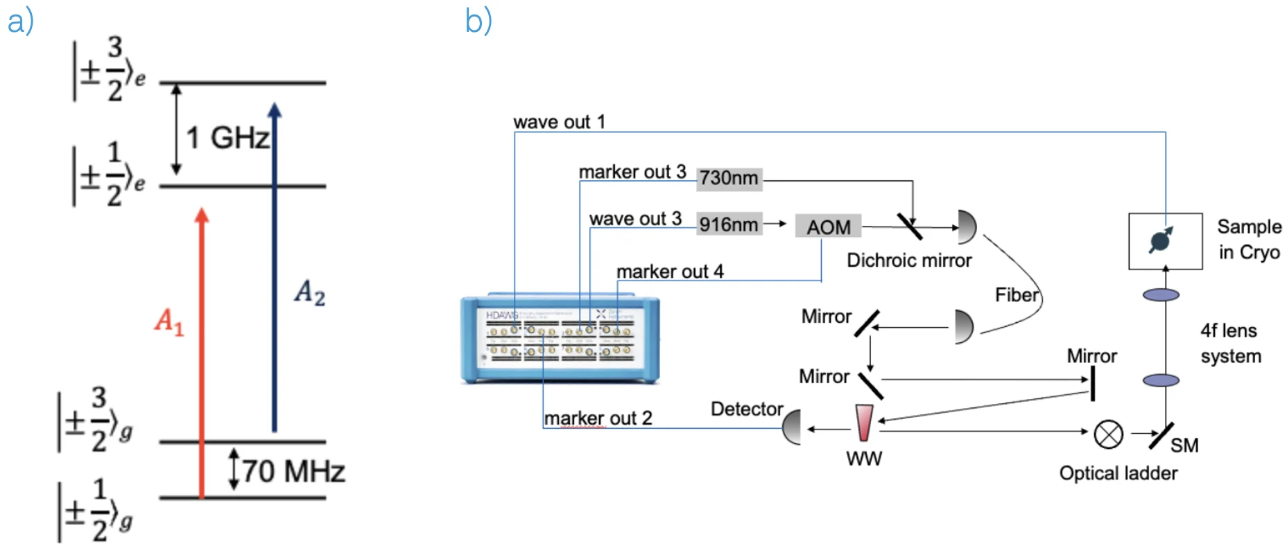
Experimental Setup

The DUT is placed in a cryostat at 4K with a home-built confocal microscope. A 730nm laser is used for off-resonant excitation and a 916nm laser for resonant excitation. An acousto-optical modulator (AOM) is used to pulse the 916nm laser. The wavelength of the 916nm laser is tuned through a DC voltage, where the wavelength of the laser can be measured with a wavemeter. The excitation light is reflected at a scanning mirror (SM) and focused on the DUT inside the cryostat. The fluorescence is forwarded to a superconducting nanowire single photon detector (detector). A Time Tagger Ultra from Swabian Instruments is used to detect the counts from the detector. The HDAWG controls the AOM, the time tagger, generates the RF signal for the transition between the two spin-dependent ground states, and tunes the frequency of the resonant laser. For devices that need to be switched on and off, or triggered, we connect the HDAWG marker ports, which essentially generate a high or low voltage level. For devices that need analog voltage values, we connect the HDAWG wave ports.

PLE Spectroscopy

In this experiment, we aim to measure the transitions A₁ and A₂ using the technique of PLE [1]. When the wavelength of the resonant laser matches that of the transitions, the spin-dependent excited states will be populated, leading to a photoluminescence (PL) signal.

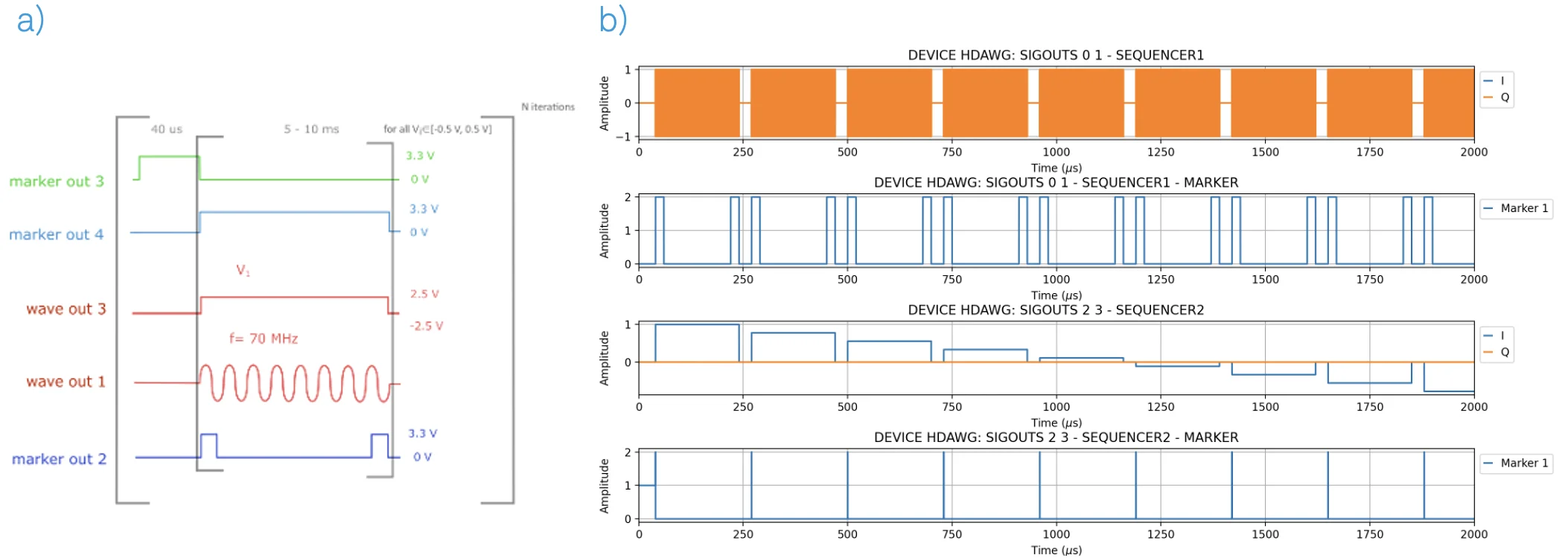
After finding a color center by using the confocal microscope control in the Qudi graphical interface, the PLE spectroscopy experiment is performed on the targeted color center. The PLE sequence is illustrated in Fig. 2a. Each line corresponds to an output of the HDAWG. Each shot starts with a 40us pulse for the off-resonant laser to ensure the correct charge state (marker out 3). After that, the resonant laser and the drive tone for the two spin ground states are turned on. The wavelength of the resonant laser is tuned by setting different voltage values on wave out 3. A 70MHz signal is applied in parallel to the voltage sweep to address the transition between the two spin ground states (wave out 1). The marker out 4 controls the AOM. The start and stop of the time tagger are triggered with the marker out port 2.

The sweep parameter of this experiment is the wave out 3 voltage that sets the on-resonant laser wavelength. This parameter is swept in a near-time loop. To ensure a precise measurement of the resonant laser wavelength, the wavelength data at the wavemeter is inquired at every voltage step using the near-time callback functions.

Once the sequence is programmed in a Labone Q experiment, we can use the plot_simulation() to illustrate the sequence in python. Fig. 2b shows the sequence programmed in Labone Q. We can recognize the 70 MHz signal for driving the transition between the lowest two levels, the marker signals for triggering the time tagger, the voltage steps for sweeping the laser frequency, and the last marker for the AOM control. This way, we know that the Labone Q experiment indeed does what we want.

Until this point, we have worked in the Labone Q emulation mode, meaning without connecting to the HDAWG hardware. Now, we can update the emulation flag, session.connect(do_emulation=False), and measure the spectrum from a color center.

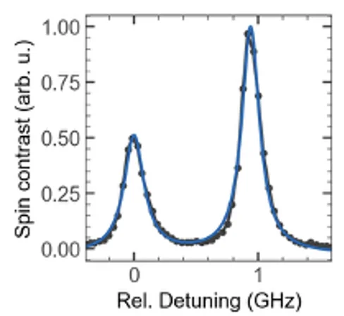
Fig. 3 shows the PLE spectrum of a V_si center in 4H-SiC as a function of the relative detuning of the resonant laser in frequency, measured with the pulse sequence from Fig. 2. The y-axis is the spin contrast, converted from the photon detector counts. A high spin contrast results from the driving of a transition. Two resonances are observed at relative detunings of 0 GHz and 1 GHz and correspond to the A₁ and A₂ transitions. A double Lorentzian curve is fitted on top of the measurement data.

Conclusion

In this blog post, the integration of Zurich Instruments' hardware into the Qudi package was demonstrated. We saw that quantum experiments such as the PLE can require complex pulse sequences. Thanks to Labone Q, the design of such an experiment becomes accessible. Together with the researchers at AQuT in Erlangen, we put the HDAWG, LabOne Q, and the integration into Qudi to the test, by recording a PLE spectrum of a cubic V_si center in 4H-SiC. In the future, it will be interesting to study how the relative spacing between the A₁ and A₂ transitions changes as a function of external electric or magnetic fields. That should provide insights of the local material properties on a nanometer scale.

Acknowledgements

We thank Ms. Kim Ullerich and Mr. Maximilian Hollendonner at AQuT for the possibility of performing these experiments, and for sharing the data and their valuable feedback regarding the blog post.

Reference

[1] D. Scheller et al. “Quantum enhanced electric field mapping within semiconductor devices”. Phys. Rev. Appl., 24, 014036, 2025.